BAGGING, BOOSTING, and RANDOM FORESTS

1. Bagging and Random Forests

Recall that bagging is a random forest with m = p. So, here is just an example of a random forest.

> library(randomForest)

> rf = randomForest(mpg ~ .-name, data=Auto)                    # By default, m = p/3. But we can also choose our own m.

> rf                                                                                          # (m is the number of X-variables sampled at each node)

Call:

 randomForest(formula = mpg ~ . - name, data = Auto, subset = Z)

               Type of random forest: regression

                     Number of trees: 500

No. of variables tried at each split: 2

          Mean of squared residuals: 8.130213

                    % Var explained: 86.53

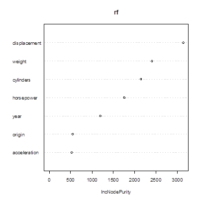
> importance(rf)                                             # Measures reduction of the node’s impurity (diversity), if split by the given X-variable

             IncNodePurity         

cylinders        2142.2611

displacement     3135.1382

horsepower       1752.5234

weight           2399.9452

acceleration      524.3148

year             1196.4857

origin            546.0370

> varImpPlot(rf)

2. Cross-validation

> Z = sample(n,200)

> rf = randomForest(mpg ~ .-name, data=Auto, subset=Z)

> Yhat = predict(rf, newdata=Auto[-Z,])

> mean((Yhat - mpg[-Z])^2)

[1] 10.19022

# The mean-square error of prediction, estimated by the validation set cross-validation, is 10.19022.

3. Searching for the optimal solution

> dim(Auto)                                                                            

[1] 392   9                                                                                           

# There are 9 variables overall in the data set, minus mpg and name = 7 variables. Let’s sample m = root of 7, rounded = 3.

> rf3 = randomForest(mpg ~ .-name, data=Auto, mtry=3)                # mtry is m, the number of X-variables available at each node

> plot(rf3)

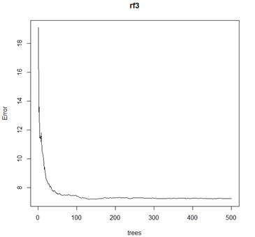
# How many trees to grow? The default is 500, but error is rather flat after 100.

# Random forest tool has multiple output:

> names(rf3)

 [1] "call"            "type"            "predicted"       "mse"           

 [5] "rsq"             "oob.times"       "importance"      "importanceSD"  

 [9] "localImportance" "proximity"       "ntree"           "mtry"          

[13] "forest"          "coefs"           "y"               "test"          

[17] "inbag"           "terms"         

# We would like to minimize the mean squared error and to maximize R², the percent of total variation explained by the forest.

> which.min(rf3$mse)

[1] 147

> which.max(rf3$rsq)

[1] 147

# Alright, let’s use 147 trees whose results will get averaged in this random forest.

> rf3.147 = randomForest(mpg ~ .-name, data=Auto, mtry=3, ntree=147)

> rf3.147

Call:

 randomForest(formula = mpg ~ . - name, data = Auto, mtry = 3,      ntree = 147)

               Type of random forest: regression

                     Number of trees: 147

No. of variables tried at each split: 3

          Mean of squared residuals: 7.322948

               % Var explained: 87.63

# This is an improvement in both MSE and R², comparing with our first random forest.

# We can optimize both m and number of trees, by cross-validation.

> Z = sample(n,n-50)                                                   # I’m choosing a small test set to make the training set close to the whole data set

> cv.err = rep(0,7)                                                       # The optimal random forest may be too dependent on the sample size

> n.trees = rep(0,7)

> for (m in 1:7){

+ rf.m = randomForest( mpg ~ .-name, data=Auto[Z,], mtry=m )

+ opt.trees = which.min(rf.m$mse)

+ rf.m = randomForest( mpg ~ .-name, data=Auto[Z,], mtry=m, ntree=opt.trees )

+ Yhat = predict( rf.m, newdata=Auto[-Z,] )

+ mse = mean( (Yhat - mpg[-Z])^2 )

+ cv.err[m] = mse

+ n.trees[m] = opt.trees

+ }

> which.min(cv.err)

[1] 7

# 7? Apparently, bagging (m=p=7) was the best choice among random forests.

> plot(cv.err); lines(cv.err)

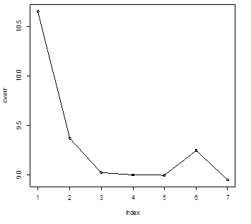
> cv.err

[1] 10.652190  9.368370  9.023726  9.000002  8.996304  9.248892  8.951198

> n.trees

[1] 112 494 318 208 484 319 293

# Result: here is the optimal random forest, which happened to reduce to bagging.

> rf.optimal = randomForest( mpg ~ .-name, data=Auto, mtry=7, ntree=293 )

> rf.optimal

               Type of random forest: regression

                     Number of trees: 293

No. of variables tried at each split: 7

          Mean of squared residuals: 7.407668

                    % Var explained: 87.81

> importance(rf.optimal)

             IncNodePurity

cylinders        4820.4219

displacement     7672.7643

horsepower       2838.2213

weight           4603.0577

acceleration      647.7559

year             2861.6324

origin            133.9062